Bresenham
Tutorial
This is to serve as a brief
overview of the Bresenham line algorithm and how it applies to image scaling.
For more detailed information or clarification, refer to
The Bresenham Line-Drawing Algorithm for the line algorithm, and to
Image Scaling with Bresenham for the scaling algorithms.
Basic Bresenham
The basic Bresenham algorithm
is used to determine which points of an n-dimensional grid should be plotted in
order to best approximate a straight line between two given points (x0,y0)
and (x1,y1). It is commonly used to draw lines on a
computer where the pixels form the raster or grid. Using integer addition and
subtraction with bit-shifting, it is a cheap and fast algorithm for
approximating lines in computer graphics. In computer programming, the x-value,
column, increases to the right, and the y-value, row, increases downward.
The goal of the algorithm is
to identify the row y that most nearly matches the actual functional value at
each column x to determine that pixel (x,y) should be plotted. The screen, a
discrete grid of pixels, forces a compromise of where we would like to draw the
pixel and the available options (only integer values). An error
results from this approximation because the mathematical point is
generally not addressable on the grid (i.e. there is no pixel at (5.23, 4.17)).
To determine which row y is
closest to the mathematical value of the function at that column x, we examine
the general line formula that follows:

We know the column x, so the row y is given by the nearest
integer to the following calculation:

We can pre-calculate the slope:

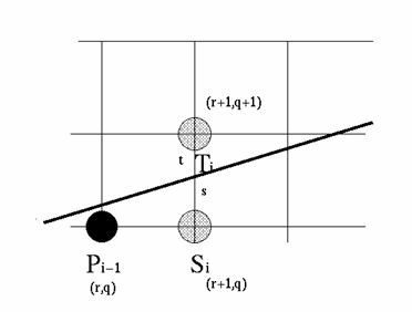
Since we assume, for simplicity, that the slope is between 0
& 1, and after rounding, we either use the previous value for y or add 1 to
it. This means we will be plotting (x+1,y) or (x+1,y+1) at every point. The
assumption about the slope is accounted for in the actual algorithm by making
adjustments to the actual values so they fit this format. This can be seen in
more detail at
The Bresenham Line-Drawing Algorithm.
To maintain the accuracy of the approximation, it is important
to track the value of the error which denotes the distance between the current
y value that is being plotted and the actual y value from the function for the
current column x. As x is incremented by 1, the error increases by the amount
of the slope (above). When the error surpasses 0.5, the line is closer to the
next y value rather than the current or previous row. In this case, we add 1 to
y and subtract 1 from the error.
Below is sample pseu docode for the Bresenham line algorithm.
function bres_line(x0,x1,y0,y1)
int changex = absoluteval(x1-x0)
int changey = absoluteval(y1-y0)
float error = 0
float changeerror = changey / changex // assume
changex != 0; i.e. line is not vertical
int y = y0
for x from x0 to x1
plot(x,y)
error = error +
changeerror
if error >= 0.5
y = y + 1
error = error - 1
end function bres_line
Bresenham for
Image Scaling
When zooming with a
Bresenham algorithm, pixels are picked up from discrete positions the
source image and placed on discrete positions in the destination image. A
common example of this is nearest neighbor sampling. When enlarging an image
with a nearest neighbor algorithm, pixels are replicated, and when shrinking
the image, pixels are dropped. Both leave artifacts in the destination images.
For a more accurate sampling,
pixels should be read from fractional positions in the source image and cover a
fractional area (rather than just one pixel) in the destination image.
Unfortunately, we are restricted to using integer values to reference pixels.
There are re-sampling algorithms that take weighted averages or nearby source
pixels to account for this fractional coverage. These algorithms are
computation-intensive and time-consuming; they would not be practical for
real-time applications. Riemersma offers smooth Bresenham scaling as a
"lightweight alternative" that creates a compromise of image quality
and processing speed.
Smooth Bresenham scaling is a
combination of linear interpolation and the coarse Bresenham scaling. The
destination pixels are set to either the value of the nearest source pixel, or
an unweighted (standard) average of neighboring pixels. This decision is
based on a threshold that is generally set to 0.5 as with the line
algorithm.
This version of an image
scaling algorithm has increased performance which is important for real-time
applications, such as zooming in and out from streaming video. This
results from the simpler calculations of using a standard average in
place of a weighted average. Also, the dropped pixel information and
excessive jagged edges of nearest neighbor algorithms like coarse
Bresenham are absent in the smooth Bresenham algorithm. That provides for
improved image quality without the problems associated with other "slow"
algorithms.
Before blindly implementing the algorithm, it is important to note how the image data is stored. With the cvLoadImage() function included with the OpenCV package, the data is placed in a one-dimensional array of bytes pointed to by a char* in the image header information. The channels or colors of the image are interleaved. The data appears as in the diagram found on the Project Progress page. Knowing that, and the fact that the Bresenham algorithm works with a single-dimensioned array of pixels, not every-third byte, some conversion was necessary. My solution here is to split the image into three one-channel images using the OpenCV function cvSplit(), run the algorithm on each separately, and re-merge the sclaed versions with the cvMerge() function. This is just one option; others may include converting the data to an array of ints where each int represents one pixel with three bytes of information (one each for red, green, and blue). I personally struggled with this conversion, but it would make a wonderful extension for this project; it could speed up the processing time even more by eliminating two calls to the Bresenham image scaling algorithm.
For more information on how
the Bresenham algorithm can be applied to image scaling, see Thiadmer
Riemersma's article
in Dr. Dobb's Journal from May 2002.
Return
to Top of Page