Coming into the first week, I had yet to come up with what exactly the project would be about. At first, I had thought a movie or video game suggestion system would be a fun topic, but decided against it in favor of football because I forgot to check recent projects before coming up with a topic. Meeting with the professors, we figured that the best course of action would be going with predicting earned points of a play based on different factors.
Week 2 (2/01/26 – 2/07/26)
The first goal that I had for this week was focusing on coming up with the project description and getting the website up and running. At this point, the concept was in place, but there wasn’t much for a question to try and answer.
The next step was getting the data from a single game, and see if I can get something close to a functional model based on the game data. The game that I decided was the matchup between the GB Packers and LA Rams in week 5 of the 2024 NFL season.
I also started to code the R programs to help clean the data. I started by using the data from the single game to make sure that the functions were working properly, before running it on the data from a whole season.
Week 3 (2/08/26 – 2/14/26)
This week was me focusing on getting the data cleaned. I was looking at getting the data from the 2021-2024 seasons all into one dataset, and then organize the play-by-play data so that it would be lined up in sequential order. It wet smoothly for the most part, the one exception being how to get kickoffs placed correctly. When a kickoff occurs, the clock doesn’t run until the ball is caught by the returner. However, if the ball goes out the back of the endzone, or the returner just takes a knee, no time is run off the clock. This means that the following play will have the same time remaining as the kickoff. At the same time, the clock doesn’t run in a game from the time someone scores, until after the ensuing kickoff. The result was a sorting list that meant I put extra points and 2-point conversions at the top of the list of plays with the same time on the clock, then kickoffs, followed by penalties/timeouts, then the list of different offensive play types.
Week 4 (2/15/26 – 2/21/26)
I started this week by finishing up the data cleaning. It was writing the few variables that help link plays to each other, even when they are not in sequential order in the dataset. The PlayID was easiest, once the data was sorted, just an incrementing value that resets when it is a new game. PreviousPlayID and NextPlayID were a little harder, as I would have to consider where I want to add the break points to not link everything together, and implement the code to do so properly. The solution that I came up with for this was that I separate the plays that I want to add previous and next IDs from those that don’t need them, before adding the values and putting the two groups back together.
Week 05 (2/22/26 – 2/28/26)
This week, there wasn’t much direct progress made on the project as a whole. A lot of work time was taken up by the increased workload that came with a take-home exam and practice for a choir concert. That isn’t to say that there wasn’t any progress made – as the in class discussions and homework for the week are important to put into practice with the capstone project as a user interface is being developed.
The topic this week was about HCI (Human-Computer Interaction). Tuesday, we looked at some examples in class, and discussed what goes into good HCI. Then there was homework for finding an example of good and bad HCI that we brought to class on Thursday. Class time Thursday was showing off these examples in a small group. We then were given an assignment over the weekend to think about HCI and apply it to our capstone project. Attached below my blog post for the week are the answers to this homework assignment.
This week had a three pronged attack to it. First, I wrote up what the values meant for each variable and documented it. Second, I started to add a dummy variable to mark the end of each drive. Third, I made the PlayID variable reset for each game, rather than just a single incrementing variable.
For writing up the variable descriptions, I took the file that was created through the PlayTypeUpdate and Sort R scripts and listed off all of the variables. Then, I was checking out each variable, seeing the values that it had, and what it meant. Documenting this is important, because up to this point, to see what a variable meant required doing this process every time, which quickly got repetitive.
Adding the dummy variable for the end of the drive sounds easy enough right? A new drive starts when the defense becomes the offence. That is a simple check within R. But what if there is a fumbled punt return that is recovered by the team that punted? What if there is an interception by the defense, fumbled, and recovered by the original offence? What if the same team that receives the second half kickoff had the ball to end the first half? All of these cases result in the same team being on offence, but there is a new drive. Starting with the most simple case, I check for if the team on offence and defense switch from one play to the next. If that happens, I mark the play before the two flip as the last play in the drive. The other cases weren’t able to get covered this week.
With the PlayID, how I had it before was just a value that said the row number. after the first game, this number isn’t very intuitive. My original plan was to use it as the Primary Key for the database that the data will go into. However, there is also a unique ID for games. This means that I could allow for the PlayID to reset every game, and still have the combination of the two be unique for every row. This also allows for the PlayID to me more intuitive when looking through the data. The PlayID says what play of the game is being observed, rather than just what play number of our dataset.
This week focused on finishing up the different cases for the change in drive. The key comes down to checking the PlayTypeUpdate. If a team is punting, regardless of what happens, the drive is over. If the returning team botches the recovery and the punting team recovers the fumble, then it should be considered a new drive, not an extension of the previous. Likewise with an onside kick. The previous play will always be a score, so I can check for if it was a Field Goal, Safety, Extra Point, or Two-Point Conversion. If there is a turnover, the offence and defense flip, unless there is a turnover by both teams, and the original offence maintains possession. Again, I would count the turnover as the end of one drive and the start of the next.
While writing the code to check this, I noticed an oddity in how offence and defense are listed for kickoffs. 2021 and 2022 have the team kicking on offence, but 2023 and 2024 have them listed on defense. This, along with other issues, has led to the decision between Dr. McVey, Dr. Dunbar, and myself to removing kickoffs from the dataset.
One of the odd cases when trying to filter out the fumbles was that if there was a botched snap, the play would be marked as a fumble, regardless of what happened after. I spent a good amount of time trying to figure out a way to find the solution to exclude these plays, without removing fumbles as a whole. Besides, does this look like it should be the transition from one drive to the next?
Picture from PackersWire. Article titled “What happened on botched snap between Josh Myers and Jordan Love vs. Patriots?”
Week 08 (3/15/2026-3/21/2026)
This is the week of Spring Break for St. Norbert College. Rather than take a week away from the project, there are a few goals that I am trying to work on.
Step 1 was trying to trim up the data. Currently there are 46 different columns for every observation, and over 175,000 observations. That is a lot of data, quite a bit of it is redundant. As seen in the list of variables from a few weeks prior, there are a few variables that don’t tell us anything. There are others that have multiple variables telling the same information. Many of the rows are also information that can be dropped. Both of these will help shrink the size of the final file and speed up calculations.
Step 2 was an extension of step 1. When going through and seeing what data was getting passed over by all the cleaning and getting thrown out at the end, there were a few play types that I would still like to keep getting ignored and tossed out. First was the spike: a play that is used like a timeout in how it stops the clock and gives the offence a chance to slow down and talk about the next play. However, this is still an official play, as it takes a down and is officially recorded as an incomplete pass on the stat sheet. Considering that I accounted for quarterback kneel plays already (which is when a quarterback intentionally gives himself up to keep the clock running with the similar tradeoff of losing a down to do so), I’m surprised it took this long for me to catch this. The other case is one that I forgot to account for, and the original PlayType variable had nothing for – a direct snap to a player that isn’t the quarterback. How I had the script written before, these plays had a full description in PlayTypeUpdate. Finally figuring out that there was a trend with these plays, I created a category for them. After this, I ran everything again and got those two types of plays fixed and part of the dataset.
Similarly, step 3 is a continuation from step 2. I was already going through and updating some of the earlier written code, so I might as well make it as streamlined as possible. Originally, the PlayTypeUpdate ran where it rewrote the original file, but the user had to select the file they wanted to do, and only could do one at a time. I made it so that it would run all the files automatically, but now it writes a new file. Writing a new file does remove some file manipulation for rerunning the code, as the process used to be that I would close down the program, delete/rename the cleaned file folder, and copy the raw data folder to rename to the name of the cleaned data folder. Then I could reopen the program and run the code. Now, the program can just run without all the workaround.
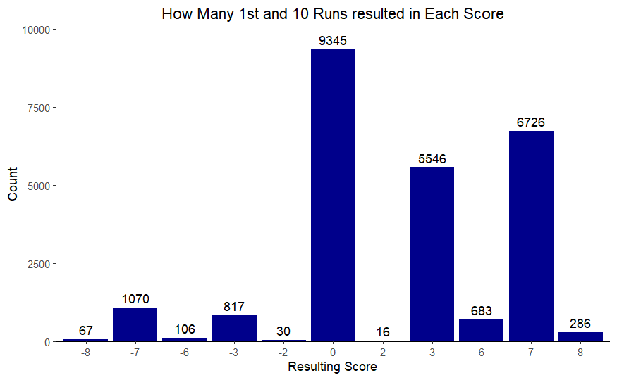
The main goal and final step is to try and start working on seeing the expected points for a given situation. The “test” case that is being used is “What is the expected point value for a team that decides to run the ball on 1st and 10?” Being able to get this filter up and running allows for my project to have the framework for filtering by down and distance and type of play. I know it isn’t much, but it is a starting point. From this, it wouldn’t be much harder to add location on the field, what team, or compare runs to passes/different types of plays.
The graph shown below is taking all of the 1st and 10 runs and seeing how many points came from the resulting drive. The most frequent result is that the team’s drive stalls out and they don’t score. It is surprisingly unlikely that the result of the drive is a turnover that has the opponent score.
Following that, I went and tried to code a simple dashboard to start doing some other exploratory data analysis. This was first and foremost to get me a little further ahead and to get a better grasp on what is needed for the rest of the project. It also had the added benefit of showing me some missing pieces within the data, or some things that might need to see some changes before moving on.
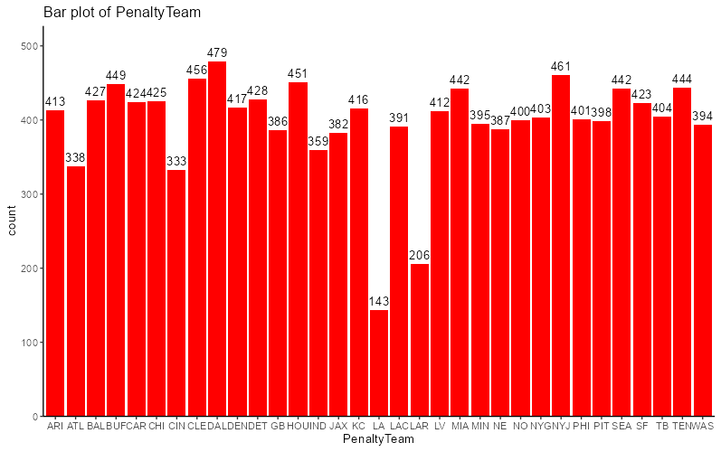
First was some of the Boolean variables. currently, they were true/false, where unless what was in them is true, they were marked as false. This becomes an issue when (for example) a simple bar graph of counts showed that there were only about 300 successful 2-Point Conversion attempts out of over 500,000. That looks like going for two following a touchdown is a silly idea. However, when we switch the values of IsTwoPointSuccessful to be empty if the play isn’t a 2-Point Conversion, all of a sudden, the conversion rate goes from <0.002% to nearly 60%. That isn’t because teams are suddenly that much better at it. It’s because the graph is no longer accounting for the plays that it shouldn’t be. I made a similar update to a number of other similar Boolean variables that only make sense to have values in certain situations. I also came across a situation shown below.
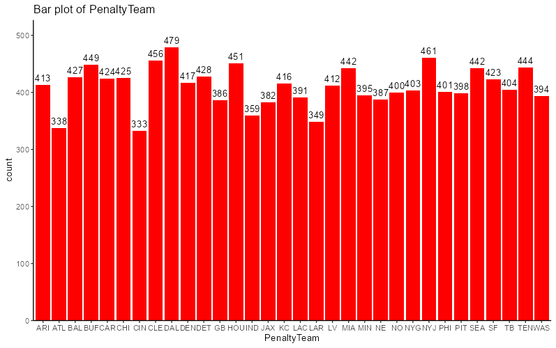
From first glance, this looks like two teams have substantially less penalties called against them than the rest of the league. This type of bias would certainly get called out within a 4 year timeframe, so why is it going unnoticed? Well, it is a lot simpler than that: looking closer into what two teams are receiving fewer penalties, they are the LA Rams and… LA…? Turns out there was some inconsistency with recording the information. Looking closer into this, between the years of 2022 and 2023, the data switches over between the two. Those two bars each account for two years of penalties, and are being compared with the other teams penalties across four years. After fixing up this inconsistency, the result looks a lot better, the LA Rams are still one of the least penalized teams, but it doesn’t look like an outlier.
Week 09 (3/22/2026-3/28/2026)
Following Spring Break, I am feeling a lot better about my project and where it is sitting than I did before. There was one key goal that I was given to accomplish this week: build on what I had last week, being able to filter for team and field position, while including both passing and running.
The task sounds simple enough, something that I was grateful for with a busier week outside of classes. The team filter would be done using the OffenseTeam variable, and the field position using the YardLine variable. It was decided that the field position will be split into five equal sections of 20 yards, because then two of the five sections will be the two red zones, a very important area of the field when trying to split up information by field position.
Passing vs Running is even easier of an inclusion. Rather than filter the PlayTypeUpdate to look for “RUSH”, have it look for “PASS”.
When putting the concept into practice with my test dashboard however, it was a lot trickier than it sounded, at least the yard line portion. Offensive team was just filter for a certain string in the column, that was ready to go in 5 minutes. Setting up the ranges for the yard line check was a little more challenging: having to create my own names for the dropdown variables and assign the values that the computer sees, and then parse values to filter the YardLine variable to be between.
When doing this though, the table I had designed would never show up, sometimes with an error attached about how the data wasn’t 2 dimensional. I decided to wait to meet with Dr McVey and Dr Dunbar to try and figure this out together.
Week 10 (3/29/2026-4/04/2026)
I had the meeting with Dr McVey, and boy was it a good thing that I waited…
The two of us had spent an hour trying what felt like every combination of different lines of code being replaced or commented out to try and manually debug what the issue was. After all of that, we were able to get the dashboard to no longer be throwing errors, and have all the buttons and filters responding correctly. However, the response given was still only on the console window of R Studio, rather than on the dashboard directly. That being said progress was still being made.
The issue that was throwing the error was found to be how the data being passed to the filters was being read in. I had it so that there was a parse function that took in the passed value, and split it to the different numbers. What needed to be done was adding an intermediate step, as R didn’t like parsing that passed variable. By instead saving the passed variable, followed by immediately using the saved variable to parse what was passed, everything ran smoothly.
Later that day, I went back through and tried to fix the issue with the table not wanting to build. I was trying to use the DataTable package tables, as they are generally better looking and have more functionality, but that doesn’t matter if there is no table wanting to show up. After scouring the internet for a solution to make a dynamic table for the dashboard, I came across the solution of renderTable() in the Server with the tableOutput() listed in the UI section of the code. Up to this point, I was trying plotOutput() in the UI and renderDT() in the Server.
Fixing that and getting a table to show up didn’t come without it’s own problems. I was testing unassumingly, with all of the variables sitting around when I got the table to work. I may have forgotten to mention that the default for the method I am using to print the table is to try and print everything. On my first run, this meant that my computer slowed to a halt trying to get this table drawn the best that it can. After I was able to regain enough control to close down the dashboard, I went to go and change the number of rows and columns that were displayed to be within an amount that doesn’t slow my computer down when rendering.
After I was able to test without my computer overworking itself, I went and added more filters surrounding Down, Distance, and Run vs Pass. None of these were any real challenge, as the framework was already in place from the other filters. I did make a quick adjustment to allow for multiple choices to be selected for many of the filters, thus giving the user more options.
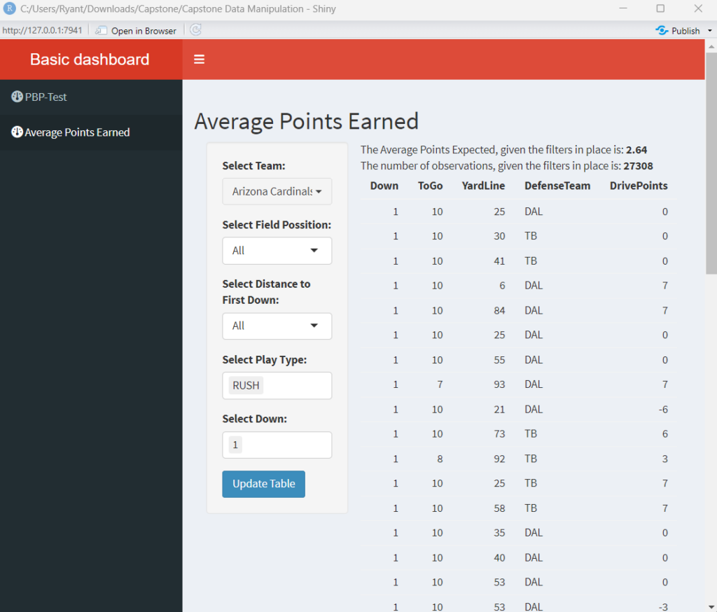
With the table, I also added some text that does the calculation for the Expected Points Added given the filters in place. At the same time as the table is told to update, the text is told to update, and part of that includes a calculation of the value, and then lists a count of how many datapoints are part of the calculation. By the end of all of the changes, it looks something line this:
The team selection is a multi-select where it has functionality to select (or deselect) all, and search for the team wanted. It was suggested to me when having Hannah test that there should be the full team names, rather than the 2 or 3 letter abbreviations that can be seen in the table. Field Position is a selection where it can be a certain 20 yard chunk described in a word or two, or the selection of all to have the filter effectively turned off by not filtering anything out. Similar is the case for distance to first down. Selecting play type allows for the selection of Run, Pass, or both. Neither is technically an option, but it filters out everything from the calculation. Selecting down is similar to play type, where any combination of 1st, 2nd, 3rd, or 4th can be selected to show the data on the representative down, but not having one selected filters out all of the data.
Week 11 (4/05/2026-4/11/2026)
This week we had our second presentation with the group. I spent most of the week getting ready for this, wanting to do the best I could to show off the work I have done the last two and a half months. The goal of my meeting was to highlight the dashboard that I have been building the past month to test variables on the fly, and to let the audience choose what was being displayed during the presentation. I wanted to make this a test run of the big event in a few weeks. The notes that I used to help guide my presentation can be found at the end of this weeks blog post.
There was some helpful feedback that I got on how to move forward with the project as a result of the presentation. Specifically looking at switching to a different display (such as a chart or graph rather than table), clarifying the part where negative means opposing team scored points on the next drive, the ability to see the results of specific plays (something like adding yards column and play type column), and adding a way to compare between queries. I really want to get at this last one, as I feel like it would be a very important aspect of why people are visiting the website. Being able to compare the results calculated between outcomes helps add a lot more context to the impact on certain decisions.
When talking with Dr Dunbar about the presentation I had last week, another implementation that could be added based on the results of the play is if it result of the play was a first down or score. I will be working on getting that and the ability to compare results, but otherwise my time will be spent converting the dashboard that I have from R shiny into the Flask / HTML that our final product is supposed to be in.
The first down/score check can be a variable in the dataset, so that will be added using R, but I don’t intend to add the comparison feature to the R shiny dashboard, but will try to add it once things are converted. The question is when we check for if a team scores when checking the result of the play, what types of scoring should be included? On scores that aren’t touchdowns or safeties, what is the play that got them the score? It feels wrong to include an incomplete pass on 3rd and long to be a play that a team got the score on because there is a Field Goal on 4th down, but it feels too obvious to say the Field Goal is the play that got the score.
The finish line is definitely in sight, and approaching way quicker than I would like to admit. I certainly wish I would be able to keep improving what I have to include all of the suggestions, but I need to turn my attention from “what can still be improved”, to “make what I currently have presentable”.
Week 13 (4/19/2026-4/25/2026)
Step 1 to getting the dashboard from R Shiny to Python/HTML was looking into the file that the Data Capstone students were given from Dr McVey for the flask project looking at reading in csv file and different methods of filtering through it to create a graph.
Once I had that online, I went and altered the code so it was reading in a variable from my dataset, rather than one from the sample provided. My reasoning was that once there was one variable implemented, it would be so much easier to get additional variables implemented.
That’s exactly what was next. Get it so that I was looking at the same filters as I had on the R shiny dashboard. I had started with the Team dropdown, so that was already in place. The Down multiselect was an easy implementation, but was manually written in because 0 was showing as an option. This will be revisited later to see if there is a problem with string vs integer for variable type when filtering. Adding YardLine and ToGo were’t much harder, but the bins that I used weren’t in order like I had hoped. Luckily, there is a simple function within pandas that would take care of that. I just had to make sure to implement the sort before I went and created the bins, as then the bins would go over the values. If I wait until the bins were created to sort, they would show up in alphabetical order, which isn’t as helpful or intuitive. I also wrote in the Play Type manually, as there are several play types that are getting excluded (i.e. Punt, Kickoff, and Field Goal). I see this being less of a potential problem than Down, as it would be a string in either situation.
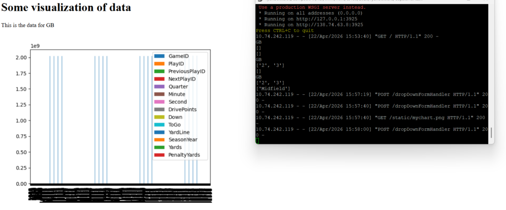
However, there were some issues with how I broke up the questions. They were all their own form, which wouldn’t work when trying to get responses from them. I was able to merge them all together into a single form and then make it so the submit button grabbed all of the information before passing it on. At the moment, this process takes over two minutes to read the csv file and draw the graph. The information the graph is giving isn’t interpretable at this stage, but it is passing information and progress is being made!
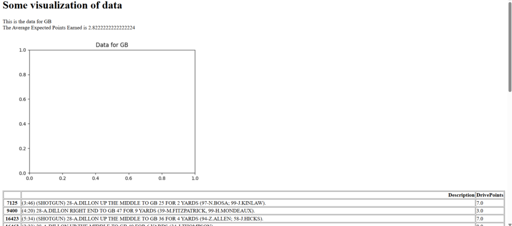
Since then, I have been able to get a table display of the plays that fit the filters passed, and calculate and display the average Expected Points Earned. At this point, the Flask is looking similar to what I had for the R shiny Dashboard at the time of our walkthroughs a few weeks ago. Now all I need to do is get the filters to show, and to save the results to roll over for comparison.
Week 14 (4/26/2026-5/02/2026) PRESENTATION WEEK
This week has two goals:
Make sure that I can show previous results (this will naturally include showing the filters, as I need to label the values)
Practice my presentation
Right away Sunday night, I was trying different things to get a table of previous results. I was able to do this, but then when having a friend also test the website, they were seeing my previous searches, and they weren’t refreshing after I would close the session and reopen it. So the final problem came in with how do I filter to the specific device? The solution was to go with a computer specific value, and filter the table of searches for the matching value when pulling up past searches.
Meeting one final time with Dr. McVey and Dr. Dunbar on Tuesday has given me a few fixes on the results screen to try and implement. Reversing the table so that the newest result is first (or finding another way to emphasize it), adding back in the histogram and making it work for the data that I have, and adding the count for the number of plays that are selected through the filter. None of these tasks seem extremely difficult, but help make the end result that much better.
The middle of the week was spent building and polishing the presentation. Having the presentation room reserved for the group 3 hours a day for the whole week leading up has allowed for plenty of time for me to get practice in with a few of my classmates. This also provided me with some advice and an idea or two on how to improve for when I present Saturday.
I spent Friday evening polishing up my Flask website with the few changes that I was suggested by the professors. I know, a terrible idea. However, I kept the working backup the whole time, so worst case scenario was just wasting my time. I got all of the suggestions added after roughly an hour. I was then able to get some practice in on presenting, and find a few more ways to fix it for the next morning.
I was heading into the presentation nervous as can be. However, I was also feeling good about everything. I got one final test run in the Campus Ministry building next door, and had a time of 15 minutes talking to myself without the demo, which will cause for a 20 minute presentation, the perfect time to achieve.
The presentation went well overall, with a few minor hiccups. I was able to have my parents and brother come, as well as a number of other friends. Plenty of people had come up to me the rest of the morning and said what a great job I did. Some of my personal criticisms were that there was a mishap where the presentation wasn’t showing after I came back to it following the demonstration of my website. This could have been avoided if I practiced and prepared for it. However, I was able to handle this smoothly and recover fairly seamlessly. I see it as being able to show off how I was able to stay level-headed under pressure and adversity. Considering a lot of people were seeing issues with the demo, the fact that mine was that small of a nitpick is also a good feeling. I was also able to handle wone of my greatest issues with presenting better than expected as well. I don’t like to bring it up often, but I have a processing disability that causes me to take an extra second or two for a question to register before I can form a response. It is important to note that this gets better when I am comfortable with an individual or situation. My mom had come up to me following the presentation and pointed out how quickly I was able to respond to questions throughout the presentation. It isn’t something that the average viewer would notice, but it goes to show the level of knowledge that I had with the topic, as nothing else about the situation would have caused me to feel more comfortable than something like an interview.
Weeks 15 and 16 (5/03/2026-5/14/2026) Defense Week and Final Touches
The time to make last minute adjustments and defend what I have with the professors is here. I’m surprisingly excited to explain anything that I will be asked about.
I feel like the data cleaning code from R was already in a good place, everything documented well. I did take a bit of time to get the Python Flask in the same spot, cleaning up the ‘app.py’ file specifically. This mainly consisted of adding comments around sections of code that describe what each section is doing. However, there were a few lines of code that were not being used, and thus were removed. Functionally, the code is the same as what was shown on Presentation Day, but the code itself is neater.
Otherwise, before the presentation, it is just updating everything on the website and getting it ready. With my defense time being 11am on Tuesday, and having everything ready on the website 24 hours in advance, it is a quick turnaround going from Saturday morning/afternoon presenting to getting everything cleaned and ready 11am Monday, but at least I’m getting it out of the way early.
Following the Defenses with the professors, the one fix that I wanted to make was making the graph read better. Currently, it is a histogram with bars that are roughly 1 point each, but there isn’t much control that I can have on it to make the bars the same every time. Talking with Dr. Dunbar, it sounds like there is a way to import the ggplot notation into python. This would be a massive help, as I am so familiar with using it in R. This would allow me to change it to a bar graph, and to make it look so much better than I could with what is currently being used.
Other than that, all I have to do yet is get everything that I did or useful notes written down and turned in with my project to the professors. I was also tasked with trying to come up with a few potential extensions to my project in hopes that it can be expanded upon. I really enjoyed the project I had, but it was a lot of data cleaning, and didn't leave much time to do other things with the data once it was ready. Having other students build off of what was started here allows for that additional time to work with the data, while not worrying about cleaning it for 5 weeks first. All it would realistically take is an hour or less to go get the data, update the R files to include the newer years that I didn't have access to, and then run through everything.