Goal
To uncover the pitcher, batter duel, it is important to understand how pitchers utilize their pitch sequencing and command to their advantage. Pitcher's decisions depend on many factors, such as count, inning, score, runners on base, and even the specific batter they are facing.
With this level of specificity, there is not enough data for each situation to model what a pitcher would do. This does not make it possible to predict a specific outcome or what will happen in any given situation. However, utilizing a simulation allows users to see what could result from varying pitches and locations given the pitcher and batter
matchup they selected. By simulating each pitch 1,000 times, this additionally helps uncovers underlying trends in the data.
Play Ball!
Playing in the role of the pitcher, users will choose to face a left or right-handed batter for an at-bat, trying to strategicially vary their
pitch type and location to try to strike the batter out! Through this simulations, users will get to explore which locations and sequencing is most advantageous to the pitcher.
Data
I am using data scraped from MLB Statcast from the 2024 and 2025 seasons. This data contains every pitch from each regular season.
After I downloaded the raw MLB Statcast data, I created various datasets that would be used for the simulation and displaying the pitcher and pitch type options available to users. I created the following datasets to be
used in the simulation:
-
Pitcher Options: Pitchers with enough data to run the simulation
First, I had to figure out which pitchers the users could select. To do this, I took raw data from the 24 and 25 MLB seasons and created a list of pitchers that threw at least
1,000 pitches to both left and right-handed batters. This ensures users can only select pitchers who have enough data for the simulation to run.
This dataset holds the player ID number, player name, and whether they throw left or right-handed. The name and handedness of the pitcher are then displayed to the user in the dropdown menu and the
ID number is used to identify the pitcher in the other datasets.
-
Pitch Options: Types of pitches that are dynamic to the pitcher and batter stance selected
After the list of Pitcher Options has been created, I had to determine which pitches they could throw to each batter stance. For each combination of pitcher and batter stance, I only included the pitch type option if the following conditions were met:
- Each pitch type was thrown at least 50 times
- The pitch type was swung on at least 25 times
- There were at least 10 recorded takes (no swings), hits, fouls, and swing and misses for the pitch type
In order for this simulation to work, I had to make sure there was enough variability in the results for each pitch type. For example, if the batter never swung on the pitch in the raw data, the simulation cannot predict whether the batter would swing or not. Additionally, if the batter only recorded
a foul for any time they swung, the simulation would not be able to predict the likelihood of recording a swing and miss or hit.
-
Full MLB Dataset: Raw data for pitchers in Pitcher Options from the 24 and 25 seasons
Finally, I filtered the full MLB Statcast data from 24 and 25 seasons to only include rows for the valid pitcher and pitch types listed in Pitcher and Pitch Options.
Flow of Simulation
On the Play Ball! page, once the user makes all of their selections (pitcher, batter, pitch, location), and hits "Throw Pitch!" all of the following steps are run.
When the user first hits "Throw Pitch," the MLB Datasetis filtered to only rows for the pitcher and batter stance selected by the user. Data for this matchup is then used for the rest of the steps in the simulation.
-
Calculating Pitch Type Parameters
With the selected pitch type, the pitcher's data is filtered down to rows where they threw that selected pitch. Two sets of parameters are now caluclated: swing_decision and contact parameters. Both parameters use the predictors:
- dist_x: horizonal distance from the center of the strike zone (same as the horizontal location of the pitch (plate_x))
- dist_z: vertical distance from the center of the strike zone (vertical location of the pitch (plate_z) - 2.5)
- balls: number of balls in the count when the pitch was thrown
- strikes: number of strikes in the count when the pitch was thrown
I would like to note that balls and strikes are numerical, rather than categorical. These variables were originally categorical, but I encountered errors running the model due to not having enough observations and variability for each count. It was running a model for all 12 unique counts,
where many counts had fewer than 10 rows of data or all resulted in the same outcome (ex: every observation resulted in batter taking the pitch as a ball). I first tried to limit my dataset to only pitchers and pitch types that had data for each count, but this resulted in only being able to throw
fastballs for any given combination. I instead decided the better approach was to remove the categorical classification from balls and strikes. This no longer requires pichers to have enough data for each count, and still effectively captures the effects of batters being more likely to swing when there are fewer strikes
and foul on #-2 counts, for example.
Swing_decision_params uses a logistic regression model on the pitch type to determine whether the batter will swing (is_swing = 1) or not (is_swing = 0). Using raw data for the pitcher, batter stance, and pitch it fits the following model:
is_swing ~ dist_x + dist_z + balls + strikes
The coefficients of this model are stored in swing_dec_params for the pitch type and used in the
Batter Decision function.
Contact_params then filters the same data from swing_decisions to only include rows where the batter swung. It uses the following multinomial logistic regression model to determine what type of result the batter recorded from swinging:
simple_result ~ dist_x + dist_z + balls + strikes
Whiff, or swinging_strike, is the baseline of this model. The coefficients of foul and inplay are relative to whiff, and are stored in contact_params and used in the
Swing Result function.
-
Running the Functions of the Simulation
-
Find_Location
The location the user selects on the screen is converted from it's pixel coordinates to the strike zone coordinates using an affine transformation. Once transformed, the
strike zone coordinate selected is sent to this function.
This function utilizes a normal distribution. The user's selected location is the average location of the simulation, mu_x and mu_z. Each run of the simulation then takes a random, simulated x and z coordinate from this
distribution, L_x and L_z. The spread where simulated pitch locations can be taken from is based off of an estimated standard deviation for each pitcher, batter, and pitch type combination. For more information on how I
estimated the standard deviation for each pitcher, click here!
The function will first check if the simulated L_x and L_z location falls within the starndard deviation of the pitcher. If it does not, it will select a new simulated L_x and L_z until it falls in that range. Once a simulated location
passes this check, the L_x and L_z coordinates are passed to the following functions.
-
Batter Decision
Given the simulated location (L_x, L_z), current count (B, S), and the swing_decision parameters, the batter must now decide if they will swing at the pitch.
This function applies the coefficients saved in swing_decison parameters and uses them to calculate the likelihood of a swing given the simulated location and current count of the at-bat. It uses the following logistic regression model:
logit = params[intercept] + (params[b_x] * L_x) + (params[b_z] * (L_z - 2.5)) + (params[b_b] * B) + (params[b_s] * S)
where:
- params[] references the coefficients stored in swing_dec_params
- L_x and L_z are the simulated locations from Find Location. In swing_dec_params, b_x and b_z are coefficients for the horizontal and vertical distance from the center of the zone. L_x and L_z must also be translated to the distance from center.
- B, S are the number of balls and strikes in the user's current at bat simulation
The result of the logit is then passed to a sigmoid function, which maps any real number to a number between 0 and 1.
prob_swing = 1 / (1 + e^(-logit))
With this probability, the function generates a random number between 0-1. If the random number < prob_swing, then the batter chose to swing at that pitch. Each run, this function stores the batters decision (0 for no swing, 1 for swing), and the actual
prob_swing probability.
If the batter decides to swing, then the "Swing Result" function runs; if not, then the "Umpires Call" function.
-
Swing Result
If the decision from Batter Decision = 1, then the batter decided to swing. This function now determins whether the result of that swing will be a whiff (swing and miss), foul, or hit into play.
This function applies the coefficients saved in contact parameters and uses them to predict the result of the swing given the simulated location and current count of the at-bat. It utilizes a multinomial logistic regression.
First, the function calculates the multinomial predictors:
whiff = 0
foul = params[foul_int] + (params[foul_b_x] * L_x) + (params[foul_b_z] * (L_z - 2.5)) + (params[foul_b_b] * B) + (params[foul_b_s] * S)
inplay = params[inplay_int] + (params[inplay_b_x] * L_x) + (params[inplay_b_z] * (L_z - 2.5)) + (params[inplay_b_b] * B) + (params[inplay_b_s] * S)
where:
- params[] references the coefficients for foul and inplay stored in contact_params
- L_x and L_z are the simulated locations from Find Location. In contact_params, b_x and b_z are coefficients for the horizontal and vertical distance from the center of the zone. L_x and L_z must also be translated to the distance from center.
- B, S are the number of balls and strikes in the user's current at bat simulation
Whiff is set to 0 to represent the baseline category. The results of foul and inplay are now measured relative to whiff; they are more or less likely to occur than a swing and miss.
Each predictor result is then passed to a softmax function that converts the raw score into probabilities that sum to 1.
p_whiff = exp(whiff)/exponential sum
p_foul = exp(foul)/exponential sum
p_inplay = exp(foul)/exponential sum
where:
- exponential sum = exp(whiff) + exp(foul) + exp(inplay)
Now, dividing each results' exponential score by the sum of all exponential scores gives a probability for each outcome that adds up to 1. Each probability now represents the
likelihood of that outcome occuring for the specific simulated location and count.
Now, with these probabilites, the function has to choose a final outcome. Rather than choosing the most likely outcome every time, this function uses a random weighted probability. For example, let's say the simulation gave the following probabilies:
- Swing and Miss: 30%
- Foul: 50%
- Hit Into Play: 20%
The computer essentially spins a wheel and whatever it lands on is the outcome of that pitch. Since there is a 50% chance the result is a foul, it will most likely choose foul as the final outcome, but there is still a chance it will select one of the other options.
-
Umpire's Call
The batter has decided not to swing, so now the umpire has to decide whether the pitch is called as a ball or a strike based on the simulated L_x and L_z location.
To make the decision, this function compares the simulated L_x and L_z location to the bounds of the strike zone. The strike zone is defined as +- 0.7083ft from the center horizontally, and 1.5 to 3.5 ft vertically.
It first determines the distance from the edges of the strike zone and whether L_x or L_z is closer to the edge.
dist_x = 0.7083 - abs(L_x)
dist_z = 1 - abs(L_z - 2.5)
In both cases, if the result of dist_x or dist_z is negative, then the ball is outside the zone. A negative value applied to the logistic regression function below will result in a probabily close to 0, meaning it would be called a ball.
The function then uses the following logistic function:
logit = k * min_distance
where:
- k = 30; This steepness value was chosen to create a sharp boundary of the strike zone. Pitches that are just inside the zone will almost always be called a strike. Similarly, pitches just outside of the zone will almost always be called balls. As the distance from the zone increases, the transition from being called a strike versus ball
changes very quickly, which represents a very consistent umpire that follows the set strike zone well.
- min_distance is either dist_x or dixt_z, whichever coordinate from (L_x, L_z) is closer to the edge of the zone.
It applies this result to a logistic function to get a probability between 0 and 1, where 1 represents the umpire calling a strike:
prob_strike = 1/1 + exp(-logit)
To determine the final call the function then chooses a random number to compare to the prob_strike. If the random number is less than prob_strike, then the function returns 1; the umpire called a strike.
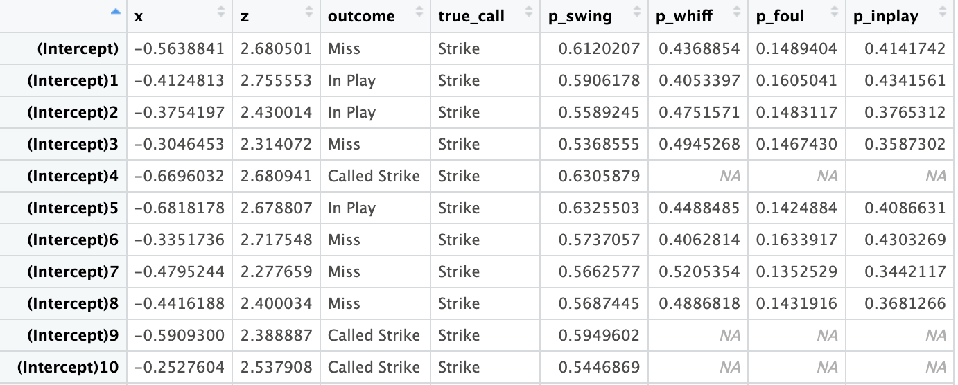
Results
For the Pitch thrown, the simulation loops through the four functions of the simulation 1,000 times. Here is a snapshot of the data stored and what it looks like:
So now what happens with this data?
First, the simulation has to choose one result from this data to display to the user. To decide the final outcome, the simulation takes a random weighted probability of all possible outcomes. This is the same method used in the
Swing Result function.
Each iteraction has an associated outcome, as seen in the snapshot above. For example, for all 1,000 iterations for one pitch, assume the following outcomes occured:
- Called Strike: 250 of 1,000 iterations = 0.25
- Ball: 450 of 1,000 iterations = 0.45
- Swing and Miss: 100 of 1,000 iterations = 0.1
- Foul: 50 of 1,000 iterations = 0.05
- Hit Into Play: 150 of 1,000 = 0.15
All possible outcomes have probabilities that sum to 1. The computer then maps each probabilty onto a 0-1 scale and generates a random number. The random number falls into the range of one of the outcomes, which is the final result displayed to the user. A Ball takes up 45% of the total probability space in this example,
so it is most likely that will be the final outcome, but it is possible for any outcome above to occur. This process mirrors the distribution of the data while allowing for outcomes other than the most probable to occur, which reflects what is seen in a real life game of baseball.
The result chosen and displayed on the screen also changes the current count of the at-bat accordingly.
Additonally, some of the data from all 1,000 iterations is displayed to the user, including:
- The likelihood of an umpire calling a ball or strike across all simulated locations. This column holds the call regardless of whether the batter swung or not.
- The average probability that a batter would swing at that location.
- The probability of any outcoming occuring. This allows users to see whether the outcome chosen was the most likely, or had a very small probability of occuring. It's possible they threw the pitch in the perfect location to maximize called strikes or misses, but the result was a hit and they got unlucky.
Together, these insights allow users to understand which locations can maximize the amount of called strikes, swing and misses, and fouls, while minimizing the number of hits.